
How to Identify Machine Learning Use Cases in Your Business
At this point, we’ve all heard of machine learning. It’s highlighted in business news, your LinkedIn feed is riddled with posts on it, and chances are

You’ve Done a Data Science, ML or AI Proof of Concept (PoC)—Now What?
While some early data science investors—like Amazon, Google and Capital One—have reaped the financial rewards by going all in on their data science in

Why Apache Spark & Azure Databricks are the Ideal Combo for Analytics Workloads
As a data scientist or a manager looking to maximize analytics productivity, you’ve probably heard—or even said—this before: “It should be done soon,

Share this content:
Resistance to change
One way or another, we have all interacted with a recommender system at some point: during Google searches, while shopping for a new book online, or even while streaming our favorite TV shows—chances are you’ve seen curated suggestions somewhere on the page.
There are several types of product recommender systems, with the most dominant variants being collaborative filtering (CF), content-based filtering (CBF), and hybrid approaches (HA). In this post, we’ll explore these variants while showing you how to implement them in practice using Keras on top of Tensorflow.
What Types of Recommender Systems Exist?
Collaborative filtering assumes that users with similar tastes in the past will have similar tastes in the future. Netflix uses a variant of CF to recommend movies and shows you might like based on similar users’ tastes in similar movies. Content-based filtering assumes that a user will like items in the future that share features—like brand, cast, genre, etc.—with items they liked in the past. Amazon uses a variant of CBF to recommend books you might want to read.
How to Identify a Dataset for a Recommender System
To build any recommender system, you need to have some data to start with. The quantity and diversity of the data you have about your products and users will define the models available to you. For example, if you don’t have product meta-data but you do have user product ratings, you can use a traditional CF model.
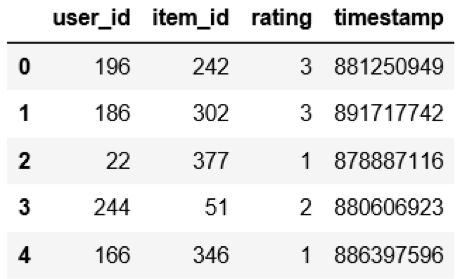
One standard recommender system dataset used as a benchmark for many state-of-the-art methods is MovieLens100K – a dataset consisting of 100,000 ratings (1-5) from 943 users of 1643 movies. However, one caveat to models based on user ratings is that they assume ratings are missing at random, or that there is no pattern to the missing reviews—but this is rarely true. Also, a user’s product preferences are based more on the actions they take—like clicking or buying—than their reviews. In response to this, a lot of recent research has pushed into implicit feedback—clicks—rather than explicit feedback—reviews. To this end, we’ll treat any rating greater than 3 as positive implicit feedback for our state-of-the-art model example.
Defining a Performance Metric for a Recommender System
Now, we’ll define how we can make progress towards our goal of recommending the right products to users. For our baseline model, we’ll try to predict a user’s rating for a given product, so we’ll use a regression metric: mean absolute error (MAE). MAE measures how close to the correct rating our rating prediction is.
For our state-of-the-art model, we’ll be classifying movies by whether a given user will react positively or negatively to it. To do this, we’ll model users’ pairwise product preferences. For each positive preference record in our data, we’ll use the movie they liked as a positive sample and randomly pick a movie as a negative sample. During model training, we can use Bayesian Personalized Ranking criterion, which pushes up the probability of recommending the positive sample, while pushing down the probability of the negative sample by adjusting model parameters. It looks like this:
positive_pair_sim, negative_pair_sim = inputs
loss = 1.0 – K.sigmoid(
K.sum(positive_pair_sim, axis=-1, keepdims=True) –
K.sum(negative_pair_sim, axis=-1, keepdims=True))
Building a Baseline Model for a Recommender System
Now that we have some data and a performance metric, we can start some modelling. We’ll start off with a simple model and gradually make it more complex. The first model we’ll construct is a traditional matrix decomposition-based CF model. The idea is to assemble your user’s product preferences into a user-product matrix, where the value at a given user + product intersection is whether the user has a positive or negative preference for that product. Then, we’ll borrow an idea from linear algebra: a matrix can be decomposed into a dot product of two vectors. In our case, we’ll model a user and a movie vector:
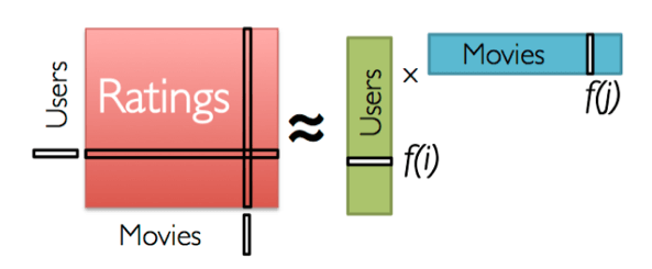
The “learning” part of this machine learning model is where we’ll gradually adjust the weights of our user vectors and movie vectors, such that when the dot product of them is taken, they represent the similarity of the user preferences to the movie’s features. We do this with both the positive and negatively sampled products: we adjust the user and movie vectors such that the positive movie vector is similar to the user vector, while the negative movie is less similar to the user vector. It looks like this:
def get_baseline_model(n_users, n_items, emb_dim=10):
user_input = Input(shape=[1], name=’user_inp’)
item_input = Input(shape=[1], name=’item_inp’)
user_embedding = Embedding(output_dim=emb_dim, input_dim=n_users + 1,
item_embedding = Embedding(output_dim=emb_dim, input_dim=n_items + 1,
#dot product layer
output = dot([user_vecs, item_vecs], axes=-1)
#define model for training and inference
model = Model(inputs=[user_input, item_input], outputs=output)
Building a State-of-the-Art Recommender System Model
To expand our model to a hybrid approach, we can take a couple of steps: first, we can add product meta-data—brand, model year, features, etc.—to our similarity measure. Next, we can add user meta-data—like demographics—to our model. We’ll then need to define how many user and item meta-data columns to use.
In this scenario, let’s say we have 5 user meta-data columns and 5 item meta-data columns. Our model will take all these inputs to its dot product similarity layer. We’ll then leverage our BPR criterion to optimize parameters of the model using gradient descent. Note : Keras doesn’t natively support this technique, so we’ll need to use a training model to optimize our parameters and an inference model to produce our similarity scores. It looks like this:
def get_sota_model(n_users, n_items, hidden_dim=64, l2_reg=0):
user_input = Input((1,), name=’user_input’)
user_meta_input = Input((1,5), name=’meta_user’)
positive_item_input = Input((1,), name=’pos_item_input’)
pos_item_meta_input = Input((1,5), name=’meta_item_pos’)
negative_item_input = Input((1,), name=’neg_item_input’)
neg_item_meta_input = Input((1,5), name=’meta_item_neg’)
history_input = Input((5,), name=’hist_input’)
l2_reg = None if l2_reg == 0 else l2(l2_reg)
user_layer = Embedding(n_users, hidden_dim, input_length=1,
item_layer = Embedding(n_items, hidden_dim, input_length=1,
hist_layer = Embedding(n_items, hidden_dim, input_length=5,
user_representation = concatenate([user_embedding, user_meta_input], name=’user_repr’)
pos_item_representation = concatenate([positive_item_embedding, pos_item_meta_input], name=’pos_item_repr’)
neg_item_representation = concatenate([negative_item_embedding, neg_item_meta_input], name=’neg_item_repr’)
positive_inputs = concatenate([user_representation, pos_item_representation], name=’pos_merge’)
positive_inputs = Dropout(0.1, name=’pos_drop’)(positive_inputs)
negative_inputs = concatenate([user_representation, neg_item_representation], name=’neg_merge’)
negative_inputs = Dropout(0.1, name=’neg_drop’)(negative_inputs)
#similarity measure layers
bpr_loss = Lambda(bpr_triplet_loss, output_shape=(1,),
inference_model = Model(inputs=[user_input, user_meta_input, positive_item_input, pos_item_meta_input],
return training_model, inference_model
Once trained, our model can be used to rank movies on how likely a given user is to react positively to them. The inference model can be called to predict a score for each movie, then the movies can be sorted according to their score and presented to the user. Over time, the more movies the user watches, the more accurate the scores will become.
Want to learn more about machine learning? Check out our blog, “ 3 Machine Learning Trends that Will Benefit Predictive Analytics ,” to learn about some of the trends we’re most excited about.
Ready to see if machine learning could benefit your organization?